Demystifying Deep Learning: Part 4
FeedForward Neural Networks
August 29, 2018
4 min read

Now to introduce our first deep learning algorithm - the feedforward neural network!
Reminder: the code for this series of tutorials can be found on GitHub.
The neuron
Intuition:
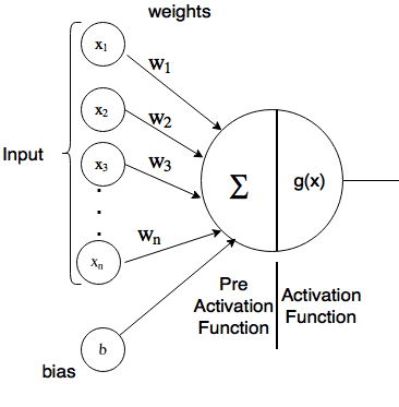
One way to look at a single neuron is like a generalised version of logistic regression - it takes in the input applying weights and a bias term, then applies a general activation function - .
Maths:
The key criterion for the activation function is that it is non-linear, since otherwise combining linear transformations would just result in another linear transformation - so a neural network would be no better than linear regression. Some terminology: We call the intermediate weighted input (before the activation function is applied) and the output (aka the activation of the neuron).
So the equations for a neuron are:
Commonly used activation functions are:
- sigmoid - (just like in logistic regression) - squashes output in range [0,1]
- tanh - this squashes output in range [-1,1].
- ReLU (Rectified Linear Unit) - - this clamps all negative values to zero, and leaves the rest of the values unchanged - it is a very simple yet highly effective activation function.
One other activation function used specifically in the output layer is the softmax function, which is used for multi-class classification problems - we will look at it in a later blog post.
Creating a Neural Network
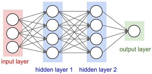
We can stack the neurons to form a layer - so all these neurons are fed the input and each outputs a prediction.
A feedforward neural network consists of multiple layers of neurons connected together (so the ouput of the previous layer feeds forward into the input of the next layer).
The first layer is called the input layer consisting of the input features, and the final layer is the output layer, containing the output of the network. The layers in between are known as hidden layers, since we can’t see their inputs/outputs.
The term deep learning comes from the typically large number of layers (the depth) of the network.
Why is this effective?
By having multiple layers, the neural network can combine input features to learn its own, more complex representation of the input in the hidden layers. The features learnt are hierarchical - i.e they build upon each other layer by layer to get more complex/abstract.
Taking our housing prices dataset for linear regression as an example, the neural network could potentially combine the “pupil-teacher ratio in area” with the “weighted mean distance to five Boston employment centres” features to create a feature indicating education, and potentially combine that in with other features like “status of population in society” and “crime rate per capita” to get a sense of the social mobility in the area.
In reality, whilst this gives intuition, it is unlikely the neural network will predict these exact features, or combine features in such a humanly-interpretable manner. Instead, it is often very difficult to interpret the weighted combinations of features used by the neural network - for the breast cancer dataset these features are nigh on impossible to interpret, given that the original data is probably hard to interpret itself.
Notation:
To keep track of all the neurons in the network, we need to add some superscripts and subscripts to our notation, and store our weights and activations in matrices.
- There are layers in our network (ignoring input) with referring to the layer in the network. We refer to the input as layer 0 and output layer as layer L.
- We are still using to denote number of examples and to denote the example - note () not [].
- The number of neurons in layer is and we store the weighted inputs and the activations for layer in x matrices and respectively. So note that .
- The input is stored in a x matrix and is a x matrix.
- The weight for layer , is stored in a x matrix - with denoting the weight between the neuron in layer and the neuron in layer .
- The bias for layer , is stored in a x matrix - one bias for each neuron in the layer.
- We collectively refer to the weights and biases as the parameters of the network.
So to give a concrete example, refers to the activation of the neuron in the layer for the example, which we store in .
Intuition:
The linear and logistic regression algorithms that we trained in the previous blog posts can be seen as tiny neural networks with no hidden layers and one neuron in the output layer, with the activation functions and respectively.
So this leads us very nicely into a much larger neural network - it involves pretty much the same operations, just at scale.
Maths:
Let’s look at the equation for this neuron - it takes input from all the previous layer ’s neurons:
In terms of the matrices:
The identity applies:
so the matrix equations are:
Notice how this is just a generalisation of our logistic regression equation to more layers and neurons!
Weight initialisation:
One key point to note is that if the neurons start off with same weights, then their inputs and outputs are going to be identical - since they’ve scaled the input from the previous layer by the same weights. This means that by symmetry they are the same, and so will be updated by the same amount.
So if all our weights are initialised to the same value, then it means that all neurons in each layer act the same. So we wish to break the symmetry which is why we initialise them randomly.
There is also another reason to initialise the weights randomly. For linear and logistic regression, the cost function is a convex surface - i.e. there is one global minimum value where the gradient is zero (think of it like a bowl). However the cost function surface for neural networks has many local minima, which may be much worse than the overall global minima (the best value) - think of this like a mountainous surface with many peaks and troughs (see image at start of post). One of our concerns is that the neural network may get stuck at the awful local minima, since the gradient is zero and therefore the parameters aren’t updated. Randomly initialising the weights allows the neural network to start at different positions on the surface, thus preventing it from getting stuck in the same minima.
So one tip when debugging your network is to run it again with different weights, and tweak the variance of the distribution from which you are choosing the weights.
Code:
def sigmoid(z):return 1/(1+np.exp(-z))def relu(z, deriv = False):if(deriv): #this is for the partial derivatives (discussed in next blog post)return z>0else:return np.multiply(z, z>0)def initialise_parameters(layers_units):#layers_units is a list consisting of number of units in each layerparameters = {} # create a dictionary containing the parametersfor l in range(1, len(layers_units)):#initialise weights randomly to break symmetry.parameters['W' + str(l)] = 0.001* np.random.randn(layers_units[l],layers_units[l-1])parameters['b' + str(l)] = np.zeros((layers_units[l],1))return parametersdef forward_propagation(X,parameters,linear):cache = {}L = len(parameters)//2 #final layercache["A0"] = X #ease of notation since input = layer 0for l in range(1, L):cache['Z' + str(l)] = np.dot(parameters['W' + str(l)], cache['A' + str(l-1)])+ parameters['b' + str(l)]cache['A' + str(l)] = relu(cache['Z' + str(l)])#final layercache['Z' + str(L)] = np.dot(parameters['W' + str(L)],cache['A' + str(L-1)]) + parameters['b' + str(L)]#depending on if linear or logistic regression#apply activation function to final layer or notcache['A' + str(L)] =cache['Z' + str(L)] if linear else sigmoid(cache['Z' + str(L)])return cache
This equations define the neural network - to output a prediction we just go forward through the network and repeatedly compute the next layer from the previous layer. This is called forward propagation.
The learning process is the same as linear and logistic regression - we’re going to use gradient descent to learn the optimal parameters. Computing the partial derivatives is a little more involved in a neural network with many layers so we will go through it in its own post.

