Demystifying Deep Learning: Part 9

Backpropagation in a Convolutional Neural Network

Introduction

In this post, we will derive the backprop equations for Convolutional Neural Networks. Again there is a Jupyter notebook accompanying the blog post containing the code for classifying handwritten digits using a CNN written from scratch.

In a feedforward neural network, we only had one type of layer (fully-connected layer) to consider, however in a CNN we need to consider each type of layer separately.

The different layers to consider are:

• Convolution Layer
• ReLU Layer
• Pooling Layer
• Fully-Connected Layer
• Softmax (Output) Layer

If you are not already comfortable with backpropagation in a feedforward neural network, I’d suggest looking at the earlier post on Backpropagation which contains some useful intuition and general principles on how to derive the algorithm.

I’ll restate the general principles here for convenience:

• Partial Derivative Intuition: Think of $\frac{\partial{y}}{\partial{x}}$ loosely as quantifying how much $y$ would change if you gave the value of $x$ a little “nudge” at that point.

• Breaking down computations - we can use the chain rule to aid us in our computation - rather than trying to compute the derivative in one fell swoop, we break up the computation into smaller intermediate steps.

• Computing the chain rule - when thinking about which intermediate values to include in our chain rule expression, think about the immediate outputs of equations involving $x$ - which other values get directly affected when we slightly nudge $x$?

• One element at a time - rather than worrying about the entire matrix $A$ , we’ll instead look at an element $A_{ij}$. One equation we will refer to time and time again is:

  $C_{ij} = \sum_k A_{ik}B_{kj} \iff C=A.B$

  A useful tip when trying to go from one element to a matrix is to look for summations over repeated indices (here it was k) - this suggests a matrix multiplication.

  Another useful equation is the element-wise product of two matrices:

  $C_{ij} = A_{ij}B_{ij} \iff C=A*B$

• Sanity check the dimensions - check the dimensions of the matrices all match (the derivative matrix should have same dimensions as the original matrix, and all matrices being multiplied together should have dimensions that align.

Convolution Layer

Recall that the forward pass’ equation for position $(i,j)$ in the $k^{th}$ activation map in the convolution layer is:

$Z^{(m_i)}_{i,j,k}= \sum_a \sum_b \sum_c X^{(m_i)}_{i+a,j+b,c} * W_{a,b,c,k} + b_k$

Since a convolution cannot be represented as a matrix multiplication, we will just consider a single neuron/weight at a time.

Just like with a standard feedforward neural net, a nudge in the weights results in a nudge in $Z$ corresponding to the magnitude of the input $X$ it is connected to. A nudge in the bias has the corresponding magnitude in $Z$.

So considering our single neuron $Z^{(m_i)}_{i,j,k}$ and a weight $W_{a,b,c,k}$ the corresponding input is $X^{(m_i)}_{i+a,j+b,c}$ from the forward prop equation above. So:

$\frac{\partial{Z^{(m_i)}_{i,j,k}}}{\partial{W_{a,b,c,k}}} = X^{(m_i)}_{i+a,j+b,c}$

$\frac{\partial{Z^{(m_i)}_{i,j,k}}}{\partial{b_{k}}} = 1$

It helps to refer back to the equivalent neurons representation of a convolution for the $k^{th} filter$. Since the weights/bias are shared, we sum partial derivatives across all neurons across the width and the height of the activation map, since a nudge in the weights/bias will affect the outputs of all neurons.

We also average the gradient across the batch of training examples.

So the backprop equations for the weights and bias are, using chain rule:

$\frac{\partial{J}}{\partial{W*{a,b,c,k}}} = \frac{1}{m} \sum*{m*i} \sum_i \sum_j \frac{\partial{J}}{\partial{Z^{(m_i)}*{i,j,k}}}\*X^{(m*i)}*{i+a,j+b,c}$

$\frac{\partial{J}}{\partial{b*k}} = \frac{1}{m} \sum*{m*i} \sum_i \sum_j \frac{\partial{J}}{\partial{Z^{(m_i)}*{i,j,k}}}$

So the equations for the partial derivatives with respect to the weights and biases are fairly similar to that of a feedforward neural net, just with parameter sharing.

Now we need to compute the partial derivative with respect to the input $X$ so we can propagate the gradient back to the previous layer. This is a little more involved.

Firstly, note that a nudge in the input affects all of the activation maps, so we sum across the activation maps. So now let’s consider the $k^{th}$ activation map.

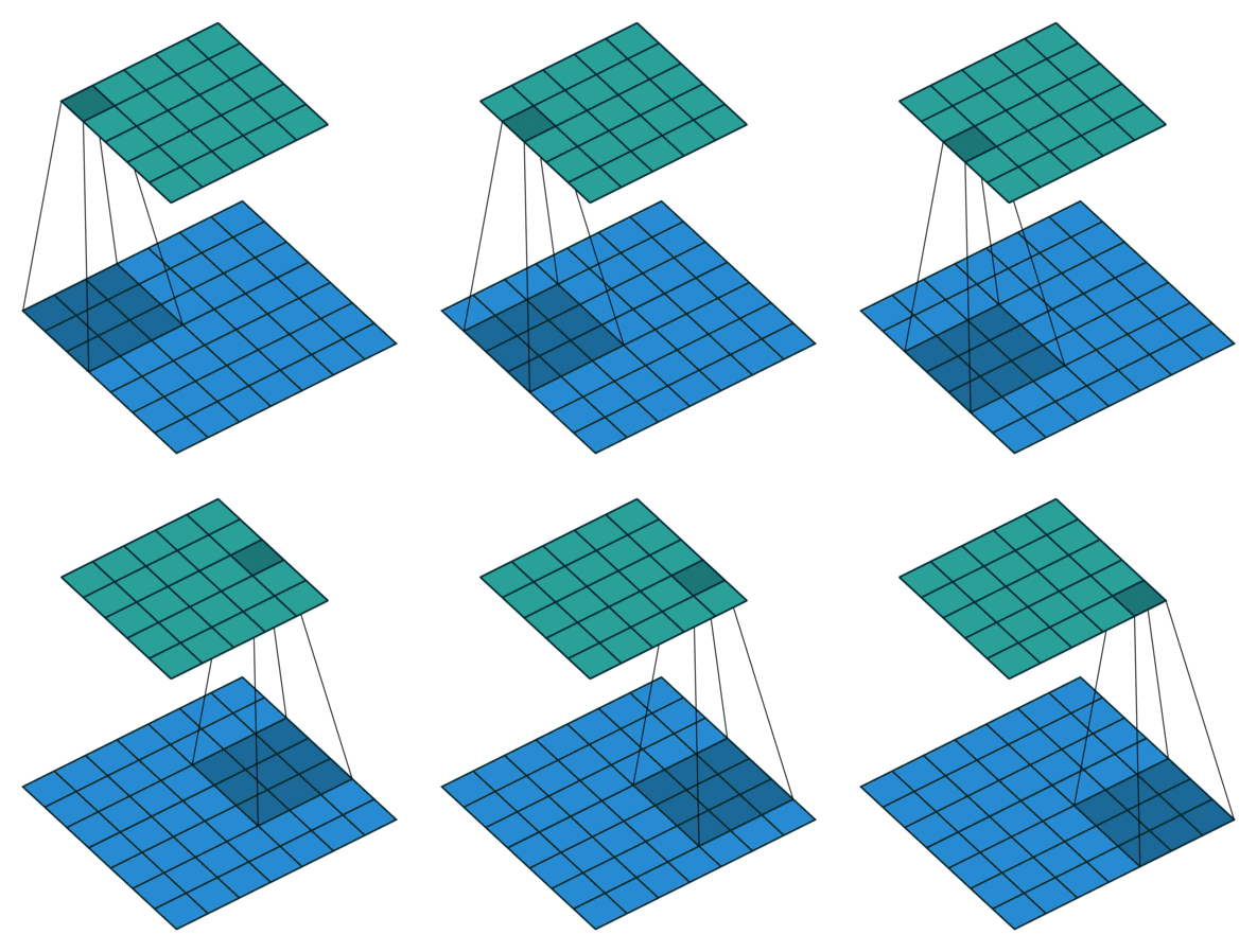
Now consider the representation of the convolution as a sliding filter operation. The filter slides over the input across the height and width dimensions so for a given input pixel $X_{i, j, c}$ , there are $F*F$ different outputs it is part of, depending on which part of the filter has scanned over it ( $F$ is the filter size). To determine the corresponding output patch when $X_{i, j, c}$ is multiplied by $W_{a,b,c,k}$ , note that in the forward pass, for $Z_{i, j, k}$ the corresponding input is offset by $(+a, +b)$ relative to the output (see equation), so from the perspective of the input, the output is offset by $(-a, -b)$ . So given an input $X_{i, j, c}$ and weight $W_{a,b,c,k}$ the corresponding output is $Z_{i-a, j-b, k}$.

So the equation is:

$\frac{\partial{J}}{\partial{X^{(m*i)}*{i,j,c}} } = \sum*k \sum_a \sum_b \frac{\partial{J}}{\partial{Z^{(m_i)}*{i-a,j-b,k}} } \* W\_{a,b,c}$

Note that this is actually itself a convolution! When implementing, we need to zero-pad the output, since around the edges, the indices (i-a,j-b) may be negative (i.e. $Z_{i-a, j-b, k}$ does not exist) - so we set these values to zero, as non-existent values shouldn’t contribute to the sum of the gradients.

Code:

When implementing, we broadcast and vectorise the operations when calculating the gradient with respect to $W$ and $b$.

def conv_backward(dZ,x,w,padding="same"):
    m = x.shape[0]

    db = (1/m)*np.sum(dZ, axis=(0,1,2), keepdims=True)

    if padding=="same":
        pad = (w.shape[0]-1)//2
    else: #padding is valid - i.e no zero padding
        pad =0
    x_padded = np.pad(x,((0,0),(pad,pad),(pad,pad),(0,0)),'constant', constant_values = 0)

    #this will allow us to broadcast operations
    x_padded_bcast = np.expand_dims(x_padded, axis=-1) # shape = (m, i, j, c, 1)
    dZ_bcast = np.expand_dims(dZ, axis=-2) # shape = (m, i, j, 1, k)

    dW = np.zeros_like(w)
    f=w.shape[0]
    w_x = x_padded.shape[1]
    for a in range(f):
        for b in range(f):
            #note f-1 - a rather than f-a since indexed from 0...f-1 not 1...f
            dW[a,b,:,:] = (1/m)*np.sum(dZ_bcast*
                x_padded_bcast[:,a:w_x-(f-1 -a),b:w_x-(f-1 -b),:,:],
                axis=(0,1,2))

    dx = np.zeros_like(x_padded,dtype=float)
    Z_pad = f-1
    dZ_padded = np.pad(dZ,((0,0),(Z_pad,Z_pad),(Z_pad,Z_pad),
    (0,0)),'constant', constant_values = 0)

    for m_i in range(x.shape[0]):
        for k in range(w.shape[3]):
            for d in range(x.shape[3]):
                dx[m_i,:,:,d]+=ndimage.convolve(dZ_padded[m_i,:,:,k],
                w[:,:,d,k])[f//2:-(f//2),f//2:-(f//2)]
    dx = dx[:,pad:dx.shape[1]-pad,pad:dx.shape[2]-pad,:]
    return dx,dW,db

ReLU Layer

Recall that $ReLU(x) = max(x,0)$ . When $x>0$ this returns $x$ so this is linear in this region of the function (gradient is 1), and when $x<0$ this is always 0 (so a constant value), so gradient is 0. NB the gradient at exactly 0 is technically undefined but in practice we just set it to zero.

Code:

def relu(z, deriv = False):
        if(deriv): #this is for the partial derivatives (discussed in next blog post)
            return z>0 #Note that True=1 and False=0 when converted to float
        else:
            return np.multiply(z, z>0)

Pooling Layer

For the pooling layer, we do not need to explicitly compute partial derivatives, since there are no parameters. Instead we are concerned with how to distribute the gradient to each of the values in the corresponding input 2x2 patch.

there are two options:

• Max Pooling
• Average Pooling

Max Pooling:

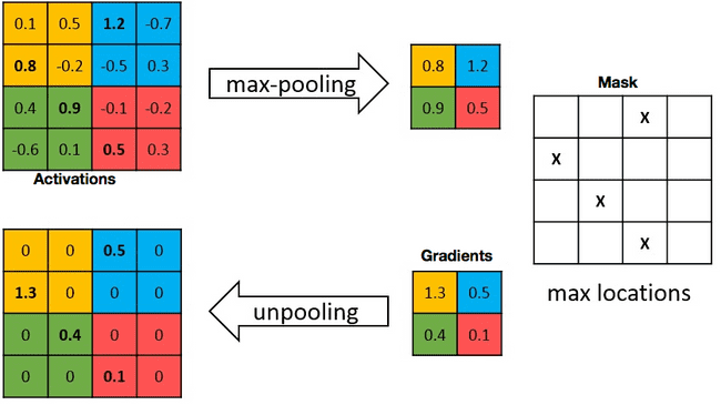
Intuitively a nudge in the non-max values of each 2x2 patch will not affect the output, since the output is only concerned about the max value in the patch. Therefore the non-max values have a gradient of 0.

For the max value in each patch, since the output is just that value, a nudge in the max value will have a corresponding magnitude nudge in the output - so the gradient is 1.

So effectively, we are just routing the gradient through only the max value of that corresponding input patch.

Average Pooling:

Here for a given 2x2 patch $X$ the output $Z$ is given by the mean of the values i.e:

$Z = \frac{X*{11}+X*{12} + X*{21} + X*{22}}{4}$

Thus a nudge in any of these values in the patch will have a output nudge that is only a quarter of the magnitude - i.e. the gradient here is 0.25 for all values across the image.

Intuitively think of this as sharing the gradient equally between the values in the patch.

Code:

It is worth bringing up the code from the forward pass, to detail how the mask, which is used to allocate gradients, is created.

Max Pooling:

We use np.repeat() to copy one ouput value across the corresponding 2x2 patch (i.e. we double the width/height of the output) - so it has the same dimensionality as the input.

To get the position of the max element in the patch, rather than doing an argmax, a simple trick is to elementwise compare the input with the scaled up output, since the output is only equal to the max value of the patch.

One subtlety with floating point multiplication is that we can get floating point rounding errors, so we use np.isclose() rather than np.equal() to have a tolerance for this error.

We then convert the mask to int type explicitly, to be used in the backward pass - so it zeros the gradient for the non-max values.

Average Pooling:

Here the gradient is just 0.25 for all values, so we create a mask matrix of the same dimensionality of all 0.25s.

For the backward pass, we scale the gradient matrix up by copying the value of the gradient for each patch to all values in that 2x2 patch, then we allocate gradients by applying the pre-computed mask in the forward pass.

def pool_forward(x,mode="max"):
    x_patches = x.reshape(x.shape[0],x.shape[1]//2, 2,x.shape[2]//2, 2,x.shape[3])
    if mode=="max":
        out = x_patches.max(axis=2).max(axis=3)
        mask  =np.isclose(x,np.repeat(np.repeat(out,2,axis=1),2,axis=2)).astype(int)
    elif mode=="average":
        out =  x_patches.mean(axis=3).mean(axis=4)
        mask = np.ones_like(x)*0.25
    return out,mask

#backward calculation
def pool_backward(dx, mask):
    return mask*(np.repeat(np.repeat(dx,2,axis=1),2,axis=2))

Fully-Connected Layer

The fully-connected layer is identical to that used in the feedforward neural network, so we will skip the derivation (see original backprop post and just list the equations below.

$\frac{\partial{J}}{\partial{W^{[l]}\_{jk}}}= \frac{1}{m} \frac{\partial{J}}{\partial{Z^{[l]}}}.A^{[l-1]T}$

$\frac{\partial{J}}{\partial{b^{[l]}}} = \frac{1}{m} \sum_{i=1}^{m}\frac{\partial{J}}{\partial{Z^{[l](i)}}}$

$\frac{\partial{J}}{\partial{A^{[l-1]}}} = W^{[l]T}.\frac{\partial{J}}{\partial{z^{[l]}}}$

The code is the same as the feedforward network layer, so again we’ll just list it below:

def fc_backward(dA,a,x,w,b):
    m = dA.shape[1]
    dZ = dA*relu(a,deriv=True)
    dW = (1/m)*dZ.dot(x.T)
    db = (1/m)*np.sum(dZ,axis=1,keepdims=True)
    dx =  np.dot(w.T,dZ)
    return dx, dW,db

Softmax Layer:

The equation we are concerned with computing is:

$\frac{\partial{J}}{\partial{Z^{[l]}}} = \frac{\partial{J}}{\partial{A^{[l]}}}*g'(Z^{[L]})$

The rest of the equations for the output layer are identical to the fully-connected layer, since the softmax layer only differs in activation function.

Recall that the cost function is the cross-entropy cost function:

$J(W,b) = \frac{-1}{m} \sum*{i=1}^{m} \sum*{k} y^{(i)}\_k \log(\hat{y}^{(i)}\_k)$

Again, we can consider a single output layer node - so consider the node corresponding to the $i^{th}$ training example and the $j^{th}$ class, ${a}^{(i)[L]}_j = \hat{y}^{(i)}_j$.

$\frac{\partial{J}}{\partial{\hat{y}^{(i)}\_j}} =\frac{-y^{(i)}\_j}{\hat{y}^{(i)}\_j}$

Next we consider the effect of nudging the weighted input of tehe output code corresponding to the $i^{th}$ training example and the $j^{th}$ class, ${z}^{(i)[L]}_j$.

Recall the equation for the softmax layer:

$softmax(z^{(i)[L]}\_j) = \frac{e^{z^{(i)[L]}\_j}}{\sum_k e^{z^{(i)[L]}\_k}}$

Clearly a nudge in ${z}^{(i)[L]}_j$ will affect the value of the corresponding output node ${a}^{(i)[L]}_j$ since we exponentiate ${z}^{(i)[L]}_j$ in the numerator.

However, there is another subtletly. Since the nudge affects the value $e^{z^{(i)[L]}_j}$, it will affect the sum of the exponentiated values, so it will affect the outputs of all of the ouput nodes, since the denominator of all nodes is the aforementioned sum of the exponentiated values.

Let’s consider the two cases separately.

First, let’s compute the derivative of the output of the corresponding output ${a}^{(i)[L]}_j$ with respect to ${z}^{(i)[L]}_j$- we use quotient rule since both the numerator and denominator are dependent on ${z}^{(i)[L]}_j$.

$\frac{\partial{a^{(i)[L]}_j}}{\partial{z^{(i)[L]}_j}} = \frac{e^{z^{(i)[L]}_j}}{\sum_k e^{z^{(i)[L]}_k}} - (\frac{e^{z^{(i)[L]}_j}}{\sum_k e^{z^{(i)[L]}_k}})^2 = \hat{y}^{(i)}_j(1 - \hat{y}^{(i)}_j)$

Next, consider the derivative of a different node ${a}^{(i)[L]}_m$ with respect to ${z}^{(i)[L]}_j$. Here the numerator doesn’t depend on ${z}^{(i)[L]}_j$ since we have exponentiated a different node ${z}^{(i)[L]}_m$.

So the derivative is just:

$\frac{\partial{a^{(i)[L]}_m}}{\partial{z^{(i)[L]}_j}} = - \frac{e^{z^{(i)[L]}_j}e^{z^{(i)[L]}_m}}{({\sum_k e^{z^{(i)[L]}_k}})^2} = - \hat{y}^{(i)}_j*\hat{y}^{(i)}_m$

Since $a^{(i)[L]}_m = \hat{y}^{(i)}_m$, and a nudge in $z^{(i)[L]}_j$ affects all output nodes, we sum partial derivatives across nodes, so using chain rule we have:

$\frac{\partial{J}}{\partial{z^{(i)[L]}\_j}} = \sum_k \frac{\partial{J}}{\partial{\hat{y}^{(i)}\_k}}\*\frac{\partial{\hat{y}^{(i)}\_k}}{\partial{z^{(i)[L]}\_j}}$

Again, we split into the two cases:

$\frac{\partial{J}}{\partial{z^{(i)[L]}_j}} = \frac{\partial{J}}{\partial{\hat{y}^{(i)}\_j}}\*\frac{\partial{\hat{y}^{(i)}\_j}}{\partial{z^{(i)[L]}\_j}}+ \sum_{k \neq j} \frac{\partial{J}}{\partial{\hat{y}^{(i)}\_k}}\*\frac{\partial{\hat{y}^{(i)}\_k}}{\partial{z^{(i)[L]}\_j}}$

\frac{\partial{J}}{\partial{z^{(i)[L]}_j}} = \frac{-y^{(i)}\_j}{\hat{y}^{(i)}\_j} \* \hat{y}^{(i)}\_j(1 - \hat{y}^{(i)}\_j) + \sum_{k \neq j} \frac{-y^{(i)}\_k}{\hat{y}^{(i)}\_k} _- \hat{y}^{(i)}\_j_\hat{y}^{(i)}\_k

Tidying up and combining the $j$ term with the $\sum\_{k \neq j}$ term to get $\sum_k$:

$\frac{\partial{J}}{\partial{z^{(i)[L]}\_j}} = -y^{(i)}\_j + \hat{y}^{(i)}\_j\*\sum_k y^{(i)}\_k$

Since the probabilities of $y$ across the output nodes sum to 1, this reduces our equation to:

$\frac{\partial{J}}{\partial{z^{(i)[L]}\_j}} = \hat{y}^{(i)}\_j-y^{(i)}\_j$

So wrapping up, having considered the equation for one neuron, we can generalise across the matrix $Z^{[L]}$ to get:

$\frac{\partial{J}}{\partial{Z^{[l]}}} = \hat{Y} - Y$

Code:

def softmax_backward(y_pred, y, w, b, x):
    m = y.shape[1]
    dZ = y_pred - y
    dW = (1/m)*dZ.dot(x.T)
    db = (1/m)*np.sum(dZ,axis=1,keepdims=True)
    dx =  np.dot(w.T,dZ)
    return dx, dW,db

Conclusion:

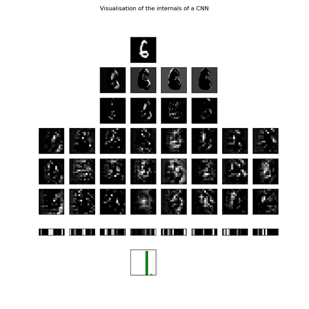
This wraps up our discussion of convolutional neural networks. CNNs have revolutionised computer vision tasks, and are more interpretable than standard feedforward neural networks as we can visualise their activations as images (see start of post). We look at the activations in more detail in the notebook.

Next we will look at another specialised class of neural networks - recurrent neural networks, which are optimised for input sequences (e.g sentences for NLP).